I gave this tutorial at the Gravitational Waves group meeting at CCA (Flatiron Institute). The whole code is available on GitHub!
The tutorial is addressed to anyone who has almost no idea of how hydrodynamical simulations on grid-based codes are constructed. My favorite examples of such codes are Athena++ and PLUTO (I’ve used them myself – I am biased).
Most of what I will be showing here is based on Michael Zingale’s textbook.
First, I just want to convince you that hydro simulations are just a work of art.
Essentially, the hydro codes just solve three Euler equations:
\[\partial_t\rho+\nabla \cdot[\rho \textbf{v}]=0\] \[\partial_t[\rho\textbf{v}]+\nabla\cdot[\rho\textbf{v}\otimes\textbf{v}+P]=0\] \[\partial_tE+\nabla\cdot[(E+P)\textbf{v}] = 0\]where \(\rho\) is the gas density, \(v\) its velocity and \(P\) its pressure.
Here, \(E\) is the specific total energy which is related to the specific internal energy as:
\[\rho E = \rho e + \frac{1}{2} \rho u^2\]and the system is closed by an equation of state:
\[P = P(\rho, e)\]A common equation of state is a gamma-law EOS:
\[P = \rho e (\gamma - 1)\]where \(\gamma\) is a constant. For an ideal gas, \(\gamma\) is the ratio of specific heats, \(c_p / c_v\).
Finite-Volume Methods
The key point of the method to discritize your fields in the way that your conservation laws hold (mass, momentum, and energy). Consider a uniform discretization of the domain \([x_L, x_R]\). The discretization will go as follows:
\[x_i = x_L+(i+1/2)\delta x\]We will also need the midpoint values:
\[x_{i-1/2} = x_i - \delta x = x_L+i\delta x\]These values define computational cells or control volumes:
\[C_i = [x_{i-1/2},x_{i+1/2})\]Cell averages are defined as:
\[U^n_i \approx \frac{1}{\delta x}\int_{x_{i-1/2}}^{x_{i+1/2}}U(x,t^n)dx\]We want to solve the following heat equation:
\[\frac{dT}{dt}-\nabla(k\nabla T) = 0\]Let’s discritize everything! We usually use $n$ for time increments and $ijk$ for spatial increments.
\[\frac{dT}{dt} = \frac{T_c^{n+1}-T_c^n}{\Delta t}\]Divergence theorem:
\[\int\int_V-\nabla\cdot(k\nabla T)dV=\int_S-(k\nabla T)dS\] \[\int_S-(k\nabla T)dS = \sum (-(k\nabla T)_i\cdot S_i)\] \[\frac{T_c^{n+1}-T_c^n}{\Delta t}+\sum (-(k\nabla T)_i\cdot S_i) = 0\]Let’s look at one of the faces. For the face \(i\), we can write (\(A_i\) is the face area, \(n_i\) is the direction of the normal):
\[-(k\nabla T)_i\cdot S_i = -k A_i n_i(\frac{dT}{dx})_i = -k A_i n_i\frac{T_E-T_c}{\delta x}\]We will call \(\frac{-kA_i}{\delta x}\) as \(f\) for the flux through that face.
In the end we will have:
\[T_c^{n+1} = T_c^n+\Delta t(f_cT_c - \sum f_iT_i)\]Example 1.
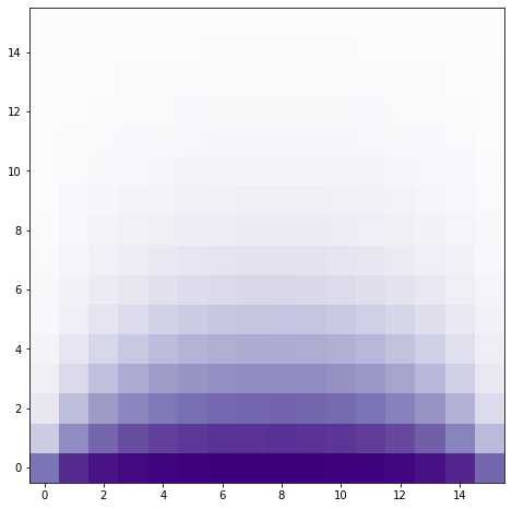
This is the example of a 1D boundary-value problem presented above. We will look at the temperature gradient in a box (it is actually a square because the equation is in 1D). Here, I put the temperature at the bottom to be \(240K\), and \(0\) everywhere else.
def FVdemo(T, imax, jmax, time, delt=0.2, k=1, FaceArea=1, dh=1):
    """
    need:
    Tc, Te, Tw, Tn, Ts
    FluxC, FluxE, FluxW, FluxN, FluxS;

    T is an NxN matrix
    delt is a delta t
    """
    Tb0 = 0
    Tb = 240
    i = 0
    j = 0
    for t in range(0,len(time)-1):
        delt = time[t+1] - time[t]
        for i in range(0,imax):
            for j in range(0,jmax):
                Tc = T[i, j];
                dx = dh;

                if (i == imax - 1):
                    Te = Tb0;
                    dx = dx / 2;
                else:
                    Te = T[i + 1, j];
                FluxE = (-k * FaceArea) / dx;

                if (i == 0):
                    Tw = Tb0;
                    dx = dx / 2;
                else:
                    Tw = T[i - 1, j];
                FluxW = (-k * FaceArea) / dx;

                if (j == jmax - 1):
                    Tn = Tb0;
                    dx = dx / 2;
                else:
                    Tn = T[i, j + 1];
                FluxN = (-k * FaceArea) / dx;

                if (j == 0):
                    Ts = Tb;
                    dx = dx / 2;
                else:
                    Ts = T[i, j - 1];
                FluxS = (-k * FaceArea) / dx;

                FluxC = FluxE + FluxW + FluxN + FluxS;


                T[i, j] = Tc + delt * (FluxC * Tc - (FluxE * Te + FluxW * Tw + FluxN * Tn + FluxS * Ts));
    return T
Example 2. Kelvin-Helmholtz instability
Here, we will create our own 2D simulation for the Kevin-Helmholtz instability!
The two-dimensional hydro equations for this flow can be written as follows:
\[\frac{\partial}{\partial t} \begin{pmatrix}\rho \\\ \rho v_x \\\ \rho v_y \\\ \rho e\end{pmatrix} + \frac{\partial}{\partial x} \begin{pmatrix}\rho v_x \\\ \rho v_x^2 + P \\\ \rho v_xv_y \\\ (\rho e+P)v_x\end{pmatrix} + \frac{\partial}{\partial y} \begin{pmatrix}\rho v_y \\\ \rho v_yv_x + P \\\ \rho v_y^2 \\\ (\rho e+P)v_y\end{pmatrix} = \textbf{0}\]Rewriting it in a matrix form:
\[\frac{\partial}{\partial t}\textbf{U}+\nabla\cdot\textbf{F(U)} = \textbf{0}\]For the equation above,using divergence theorem, we can integrate it for cell \(C_i\):
\[\frac{\partial}{\partial t}\int_{C_i}\textbf{U}dxdy = -\oint_{\partial C_i}\textbf{F}\cdot d\textbf{S}\]The cell-averaged value would be (\(C_i\) is the area of the cell):
\[\textbf{U}_i(t) = \frac{1}{\vert C_i \vert} \int_{C_i}\textbf{U}(x,y,t)dxdy\]Just like before, we will write everything in the the discritized form – this is the equation the simulation will solve:
\[\vert C_i\vert\frac{U_i^{n+1}-U_i^n}{\Delta t}=-\sum F_i\Delta S_i\]One of the important things to note here before we move further is the CFL condition (or just a Courant number condition): the distance that any information travels during the timestep length within the mesh must be lower than the distance between mesh elements. We’ll express it this way:
\(\Delta t = C\cdot min(\frac{\Delta x}{c_s+\vert v\vert})\) Second-order extrapolation in space:
\(f_{i+\frac{1}{2},j} = f_{i,j}+\frac{\partial f_{i,j}}{\partial x}\frac{\Delta x}{2}\) \(f_{i-\frac{1}{2},j} = f_{i,j}-\frac{\partial f_{i,j}}{\partial x}\frac{\Delta x}{2}\)
def getConserved( rho, vx, vy, P, gamma, vol ):
	"""Calculate the conserved variable from the primitive"""
	mass   = rho * vol
	momx   = rho * vx * vol
	momy   = rho * vy * vol
	energy = (P/(gamma-1) + 0.5*rho*(vx**2+vy**2))*vol

	return mass, momx, momy, energy


def getPrimitive(mass, momx, momy, energy, gamma, vol):
	"""Calculate the primitive variable from the conservative"""
	rho = mass / vol
	vx  = momx / rho / vol
	vy  = momy / rho / vol
	P   = (energy/vol - 0.5*rho * (vx**2+vy**2)) * (gamma-1)

	return rho, vx, vy, P


def getGradient(f, dx):
	"""Calculate the gradients of a field"""
	f_dx = (np.roll(f,-1,axis=0) - np.roll(f,1,axis=0)) / (2*dx)
	f_dy = (np.roll(f,-1,axis=1) - np.roll(f,1,axis=1)) / (2*dx)

	return f_dx, f_dy


def extrapolateInSpaceToFace(f, f_dx, f_dy, dx):
	"""Calculate the gradients of a field"""
	f_XL = f - f_dx * dx/2
	f_XL = np.roll(f_XL,-1,axis=0)
	f_XR = f + f_dx * dx/2

	f_YL = f - f_dy * dx/2
	f_YL = np.roll(f_YL,-1,axis=1)
	f_YR = f + f_dy * dx/2

	return f_XL, f_XR, f_YL, f_YR


def applyFluxes(F, flux_F_X, flux_F_Y, dx, dt):
	"""Apply fluxes to conserved variables"""
	# update solution
	F += - dt * dx * flux_F_X
	F += dt * dx * np.roll(flux_F_X,1,axis=0)
	F += - dt * dx * flux_F_Y
	F += dt * dx * np.roll(flux_F_Y,1,axis=1)

	return F


def getFlux(rho_L, rho_R, vx_L, vx_R, vy_L, vy_R, P_L, P_R, gamma):
	"""Calculate fluxed between 2 states"""

	# left and right energies
	en_L = P_L/(gamma-1)+0.5*rho_L * (vx_L**2+vy_L**2)
	en_R = P_R/(gamma-1)+0.5*rho_R * (vx_R**2+vy_R**2)

	# compute averaged states
	rho_ave = 0.5*(rho_L + rho_R)
	momx_ave = 0.5*(rho_L * vx_L + rho_R * vx_R)
	momy_ave = 0.5*(rho_L * vy_L + rho_R * vy_R)
	en_ave = 0.5*(en_L + en_R)

	P_ave = (gamma-1)*(en_ave-0.5*(momx_ave**2+momy_ave**2)/rho_ave)

	# compute fluxes
	flux_mass = momx_ave
	flux_momx = momx_ave**2/rho_ave + P_ave
	flux_momy = momx_ave * momy_ave/rho_ave
	flux_energy = (en_ave+P_ave) * momx_ave/rho_ave

	# find wavespeeds
	C_L = np.sqrt(gamma*P_L/rho_L) + np.abs(vx_L)
	C_R = np.sqrt(gamma*P_R/rho_R) + np.abs(vx_R)
	C = np.maximum( C_L, C_R )

	# add stabilizing diffusive term
	flux_mass -= C * 0.5 * (rho_L - rho_R)
	flux_momx -= C * 0.5 * (rho_L * vx_L - rho_R * vx_R)
	flux_momy -= C * 0.5 * (rho_L * vy_L - rho_R * vy_R)
	flux_energy -= C * 0.5 * ( en_L - en_R )

	return flux_mass, flux_momx, flux_momy, flux_energy

Resources:
I personally just use only these resources:
- Mike (slack)
- Mike (office)
- Mike’s textbook
- pyro – code for “easy” hydro simulations
- Finite Volume Methods for Hyperbolic Equations by Leveque
- The Physics of Fluids and Plasmas: An Introduction for Astrophysicists by Choudhuri